Deep Learning for Organic Chemistry
Utilizing Deep Learning Techniques to Identify Chemical Structures
Return to Portfolio

Table of Contents
- Question
- Introduction
- Convolutional Neural Network Model
- Hydrocarbon Training and Performance
- Small-Chain Training and Performance
- Future Work
Question
Can I build a model that can correctly classify images of chemical structures?
Introduction
Skeletal Formulas
The skeletal formula of a chemical species is a type of molecular structural formula that serves as a shorthand representation of a molecule’s bonding and contains some information about its molecular geometry. It is represented in two dimensions, and is usually hand-drawn as a shorthand representation for sketching species or reactions. This shorthand representation is particularly useful in that carbons and hydrogens, the two most common atoms in organic chemistry, don’t need to be explicitly drawn.
Table 1: Examples of different chemical species’ names, molecular formulas and skeletal formulas
| Common Name | IUPAC Name | Molecular Formula | Skeletal Formula |
|---|---|---|---|
| coronene | coronene | C24H12 | 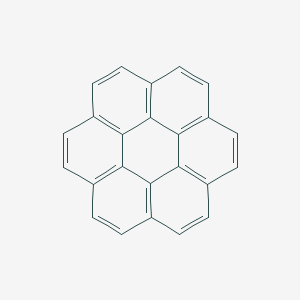 |
| biphenylene | biphenylene | C12H8 | 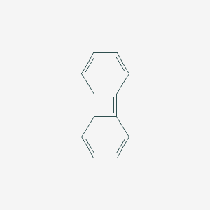 |
| 1-Phenylpropene | [(E)-prop-1-enyl]benzene | C9H10 | 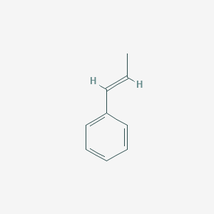 |
Simplified Molecular-Input Line-Entry System (SMILES)
SMILES is a line notation for describing the structure of chemical elements or compounds using short ASCII strings. These strings can be thought of as a language, where atoms and bond symbols make up the vocabulary. The SMILES strings contain the same information as the structural images, but are depicted in a different way.
SMILES strings use atoms and bond symbols to describe physical properties of chemical species in the same way that a drawing of the structure conveys information about elements and bonding orientation. This means that the SMILES string for each molecule is synonymous with its structure and since the strings are unique, the name is universal. These strings can be imported by most molecule editors for conversion into other chemical representations, including structural drawings and spectral predictions.
Table 2: SMILES strings contrasted with skeletal formulas
| Common Name | IUPAC Name | Molecular Formula | Skeletal Formula | Canonical SMILES |
|---|---|---|---|---|
| coronene | coronene | C24H12 |  |
C1=CC2=C3C4=C1C=CC5=C4C6=C(C=C5)C=CC7=C6C3=C(C=C2)C=C7 |
| biphenylene | biphenylene | C12H8 |  |
C1=CC2=C3C=CC=CC3=C2C=C1 |
| 1-Phenylpropene | [(E)-prop-1-enyl]benzene | C9H10 |  |
CC=CC1=CC=CC=C1 |
Perhaps the most important property of SMILES, as it relates to data science, is that the datatype is quite compact. SMILES structures average around 1.6 bytes per atom, compared to skeletal image files, which have an averge size of 4.0 kilobytes.
Building Datasets
Since all chemical structures are unique, this means that there is only one correct way to represent every chemical species. This presents an interesting problem when trying to train a neural network to predict the name of a structure - by convention the datasets are going to be sparse.
Hydrocarbon Dataset
The dataset has 2,028 rows, each with a unique name and link to a 300 x 300 pixel structural image, as shown in Table 3.
Table 3: Sample rows from the hydrocarbon dataset
| SMILES | Image URL |
|---|---|
| C=CCC1(CC=C)c2ccccc2-c2ccccc12 | https://pubchem.ncbi.nlm.nih.gov/rest/pug/compound/smiles/C=CCC1(CC=C)c2ccccc2-c2ccccc12/PNG |
| Cc1ccc(C=C)c2ccccc12 | https://pubchem.ncbi.nlm.nih.gov/rest/pug/compound/smiles/Cc1ccc(C=C)c2ccccc12/PNG |
| Cc1ccccc1\C=C\c1ccccc1 | https://pubchem.ncbi.nlm.nih.gov/rest/pug/compound/smiles/Cc1ccccc1\C=C\c1ccccc1/PNG |
Generating the image URLs required URL encoding the SMILES strings, since the strings can contain characters which are not safe for URLs. This had the added benefit of making the SMILES strings safe for filenames as well. The final training dataset was in a directory architected based on this blog post from the Keras website, where the filenames are URL encoded SMILES strings.
Small-Chain Dataset
This dataset has 9,691 rows, each with a unique name and link to a 300 x 300 pixel structural image, as shown in Table 4. It includes all of the classes from the hydrocarbon dataset, as well as new short-chain images which can include substituent atoms, such as oxygen and nitrogen.
Table 4: Sample rows from the small-chain dataset
| SMILES | Image URL |
|---|---|
| IC1CCCOCC1 | https://pubchem.ncbi.nlm.nih.gov/rest/pug/compound/smiles/IC1CCCOCC1/PNG |
| NC12CC1COC2 | https://pubchem.ncbi.nlm.nih.gov/rest/pug/compound/smiles/NC12CC1COC2/PNG |
| NCCCCC=C | https://pubchem.ncbi.nlm.nih.gov/rest/pug/compound/smiles/NCCCCC%3DC/PNG |
Convolutional Neural Network Model
CNNs take advantage of the fact that the input consists of images and they constrain the architecture in a more sensible way. In particular, unlike a regular Neural Network, the layers of a CNN have neurons arranged in 3 dimensions: width, height, depth.
Small-Data Problem and Image Augmentation using Keras
There has been a recent explosion in research of modeling methods geared towards “big-data.” Certainly, data science as a discipline has an obsession with big-data, as focus has shifted towards development of specialty methods to effectively analyze large datasets. However, an often overlooked problem in data science is small-data. It is generally (and perhaps incorrectly) believed that deep-learning is only applicable to big-data.
It is true that deep-learning does usually require large amounts of training data in order to learn high-dimensional features of input samples. However, convolutional neural networks are one of the best models available for image classification, even when they have very little data from which to learn. Even so, Keras documentation defines small-data as 1000 images per class. This presents a particular challenge for the hydrocarbon dataset, where there is 1 image per class.
In order to make the most of the small dataset, more images must be generated. In Keras this can be done via the keras.preprocessing.image.ImageDataGenerator class. This method is used to augment each image, generating a new image that has been randomly transformed. This ensures that the model should never see the same picture twice, which helps prevent overfitting and helps the model generalize better.
Image Augmentation Parameters
Keras allows for many image augmentation parameters which can be found here. The parameters used, both for initial model building and for the final architecture, are described below:
featurewise_std_normalization = set input mean to 0 over the dataset, feature-wise
featurewise_center = divide inputs by std of the dataset, feature-wise
rotation_range = degree range for random rotations
width_shift_range = fraction of total width
height_shift_range = fraction of total height
shear_range = shear angle in counter-clockwise direction in degrees
zoom_range = range for random zoom, [lower, upper] = [1-zoom_range, 1+zoom_range]
rescale = multiply the data by the value provided, after applying all other transformations
fill_mode = points nearest the outside the boundaries of the input are filled by the chosen mode
When creating the initial small dataset for model building, the following image augmentation parameters were used:
rotation_range=10
width_shift_range=0.01
height_shift_range=0.01
rescale=1./255
shear_range=0.01
zoom_range=0.01
horizontal_flip=False
vertical_flip=False
fill_mode='nearest'
Parameters 1: Initial set of image augmentation parameters for training.
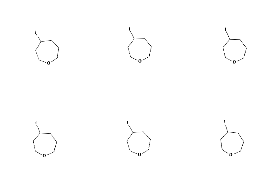
Figure 1: Sample molecule augmented using the above parameters
rotation_range=40
width_shift_range=0.2
height_shift_range=0.2
rescale=1./255
shear_range=0.2
zoom_range=0.2
horizontal_flip=True
vertical_flip=True
fill_mode='nearest'
Parameters 2: Final set of image augmentation parameters for training.
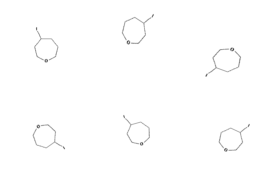
Figure 2: Sample molecule augmented using the above parameters
Model Hyperparameters
model loss = categorical crossentropy
model optimizer = Adam
optimizer learning rate = 0.0001
optimizer learning decay rate = 1e-6
activation function = ELU
final activation function = softmax
The categorical crossentropy loss function is used for single label categorization, where each image belongs to only one class. The categorical crossentropy loss function compares the distribution of the predictions (the activations in the output layer, one for each class) with the true distribution, where the probability of the true class is 1 and 0 for all other classes.
The Adam optimization algorithm is different to classical stochastic gradient descent, where gradient descent maintains a single learning rate for all weight updates. Specifically, the Adam algorithm calculates an exponential moving average of the gradient and the squared gradient, and the parameters beta1 and beta2 control the decay rates of these moving averages.
The ELU activation function, or “exponential linear unit”, avoids a vanishing gradient similar to ReLUs, but ELUs have improved learning characteristics compared to the other activation functions. In contrast to ReLUs, ELUs don’t have a slope of 0 for negative values. This allows the ELU function to push mean unit activations closer to zero; zero means speed up learning because they bring the gradient closer to the unit natural gradient. A comparison between ReLU and ELU activation functions can be seen in Figure 3.
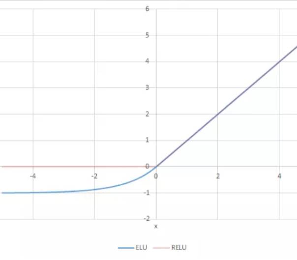
Figure 3: ELU vs. ReLU activation functions
The softmax function highlights the largest values and suppresses values which are significantly below the maximum value. The function normalizes the distribution of the predictions, so that they can be directly treated as probabilities.
Model Architecture
Sample layer of a simple CNN:
INPUT [50x50x3] will hold the raw pixel values of the image, in this case an image of width 50, height 50, and with three color channels R,G,B.
CONV layer will compute the output of neurons that are connected to local regions in the input, each computing a dot product between their weights and a small region they are connected to in the input volume.
ACTIVATION layer will apply an elementwise activation function, leaving the volume unchanged.
POOL layer will perform a downsampling operation along the spatial dimensions (width, height), resulting in a smaller volume.
The code snippet below is the architecture for the model - a stack of 4 convolution layers with an ELU activation followed by max-pooling layers:
model = Sequential()
model.add(Conv2D(32, (3, 3), input_shape=(50, 50, 1)))
model.add(Activation('elu'))
model.add(MaxPooling2D(pool_size=(2, 2)))

model.add(Conv2D(32, (3, 3)))
model.add(Activation('elu'))
model.add(MaxPooling2D(pool_size=(2, 2)))

model.add(Conv2D(64, (3, 3)))
model.add(Activation('elu'))
model.add(MaxPooling2D(pool_size=(2, 2)))

model.add(Conv2D(64, (3, 3)))
model.add(Activation('elu'))
model.add(MaxPooling2D(pool_size=(2, 2)))
On top of this stack are two fully-connected layers. The model is finished with softmax activation, which is used in conjunction with elu and categorical crossentropy loss to train our model.
model.add(Flatten())
model.add(Dense(64))
model.add(Activation('elu'))
model.add(Dropout(0.1))
model.add(Dense(1458))
model.add(Activation('softmax'))

model.compile(loss='categorical_crossentropy',
              optimizer=Adam(lr=0.0001, decay=1e-6),
               metrics=['accuracy'])
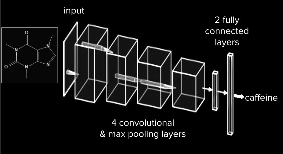
Figure 4: AlexNet style CNN architecture
Hydrocarbon Training and Performance
Training
In order to create a model with appropriately tuned hyperparameters, I started training on a smaller dataset; the initial training set had 2,028 classes, specifically chosen due to the simplicity of the structures. For each of the 2,028 classes, I used the image augmentation parameters shown in Figure 1 and Parameters 1 to train on 250 batch images per class. The accuracy and loss for this model can be seen in Figure 4 and Figure 5.
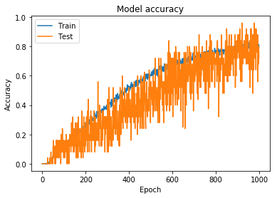
Figure 5: Model accuracy for hydrocarbon model trained using simpler augmentation parameters
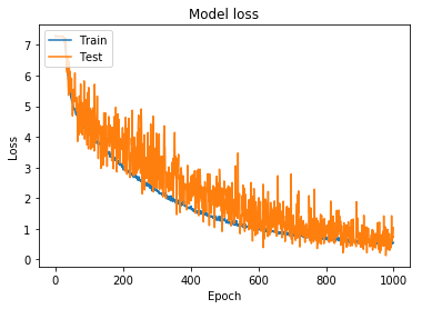
Figure 6: Model loss for hydrocarbon model trained using simpler augmentation parameters
Using the hyperparameters and weights from this training model, I started training using more difficult augmentation parameters. Since structural images are valid, even when they are flipped horizontally or vertically, the model must learn to reognize these changes. The augmented parameters can be seen in Figure 2 and Parameters 2.
The accuracy and loss for this model can be seen in Figure 7 and Figure 8.
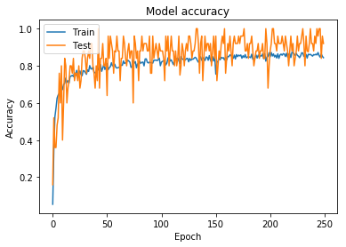
Figure 7: Model accuracy for model trained using wider augmentation parameters (including horizontal/vertical flipping)
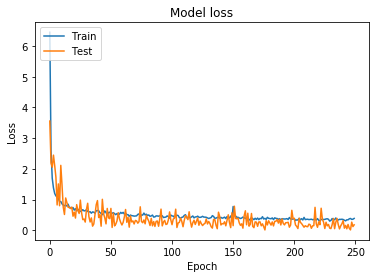
Figure 8: Model loss for model trained using wider augmentation parameters (including horizontal/vertical flipping)
Performance and Predictions
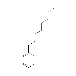
Table 5: Sample predictions from hydrocarbon model
| Image to Predict | Prediction 1 | Percent | Prediction 2 | Percent | Prediction 3 | Percent |
|---|---|---|---|---|---|---|
-c1ccc(CC=C)cc1/_0_1342.png) |
-c1ccc(CC=C)cc1/C=CCc1ccc(cc1)-c1ccc(CC=C)cc1.png) |
97.4 | 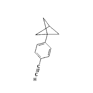 |
1.1 | c1ccccc1/C1C(=CC=C1c1ccccc1)c1ccccc1.png) |
0.5 |
Cc1ccccc1-c1ccccc1/_0_599.png) |
c1ccccc1/CC=C(c1ccccc1)c1ccccc1.png) |
61.6 | c(\C=C\c2ccccc2C=C)c(C)c1/Cc1cc(C)c(\C=C\c2ccccc2C=C)c(C)c1.png) |
33.0 | Cc1ccccc1-c1ccccc1/CC(=C)Cc1ccccc1-c1ccccc1.png) |
1.4 |
 |
-c1ccccc1/CCCCCCCCCc1ccc(cc1)-c1ccccc1.png) |
70.5 | 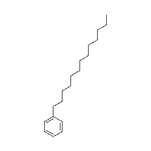 |
26.9 | 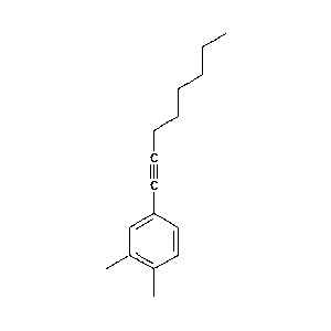 |
1.7 |
 |
 |
62.7 | 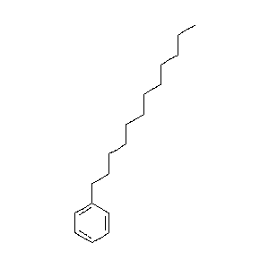 |
23.1 | 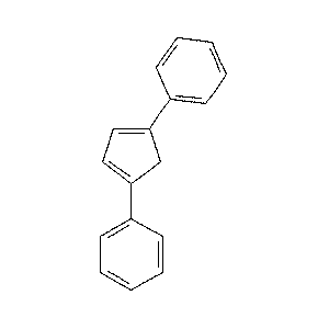 |
3.5 |
c1CCC=C/_0_802.png) |
c1CCC=C/Cc1cccc(C)c1CCC=C.png) |
85.7 | 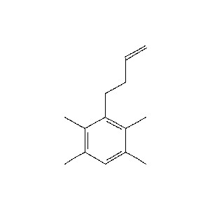 |
11.0 | 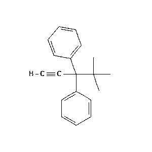 |
1.2 |
Small-Chain Training and Performance
Training
Using the hyperparameters for the 2,028 class training model, I started training the 9,691 class model. Initially, I continued using the simpler augmentation parameters. This allowed me to generate and save model weights, with the intention of eventually increasing the difficulty of the training set. The accuracy and loss for this model can be seen in Figure 9 and Figure 10.
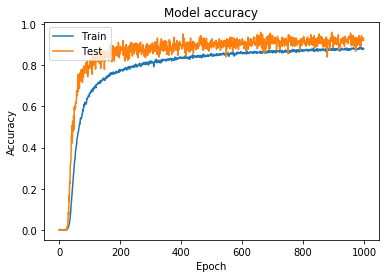
Figure 9: Model accuracy for full model trained using simpler augmentation parameters
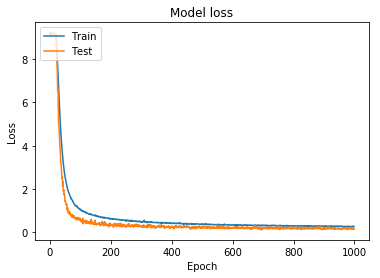
Figure 10: Model loss for full model trained using simpler augmentation parameters
I was finally able to increase the difficulty of the training set, using the augmentation parameters outlined in Parameters 2.
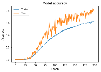
Figure 11: Model accuracy for model trained using wider augmentation parameters (including horizontal/vertical flipping)
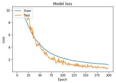
Figure 12: Model loss for model trained using wider augmentation parameters (including horizontal/vertical flipping)
While it is far from perfect, this model can predict the correct class for any molecule with upwards of 80% accuracy. Given the limitations of the datase, this is well beyond the bounds of what was expected and is a pleasant surprise.
Performance and Predictions
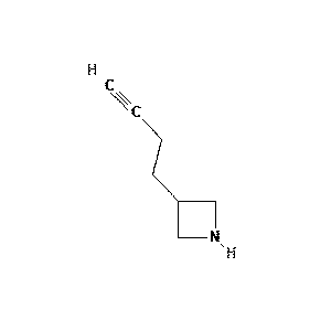
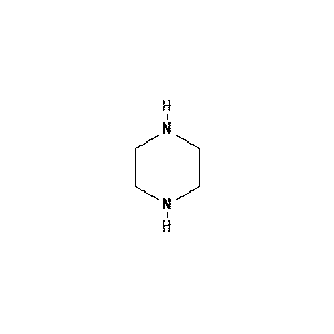
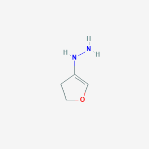
Table 6: Sample predictions from small-chain model
| Image to Predict | Prediction 1 | Percent | Prediction 2 | Percent | Prediction 3 | Percent |
|---|---|---|---|---|---|---|
 |
 |
96.4 | 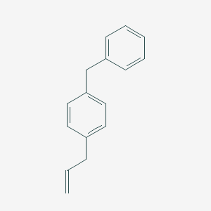 |
0.80 | 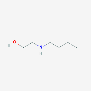 |
0.30 |
 |
 |
22.3 | 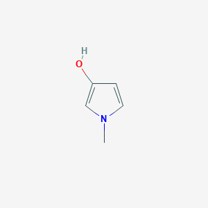 |
14.9 | 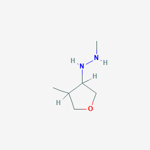 |
7.71 |
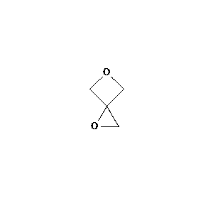 |
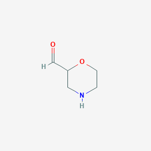 |
22.0 |  |
21.4 | 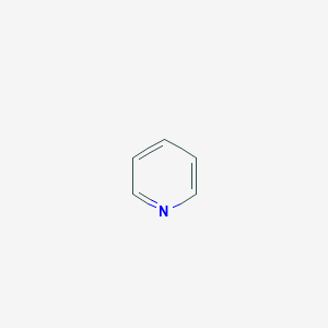 |
15.3 |
Future Work
Many of the difficulties with training my CNN could have been avoided had my dataset been larger. While the above process works, and the model has satisfactory results (can predict an image name with around 80% accuracy), the model is not generalizable. In particular, the model does not perform well (or at all) with hand-drawn structures.
In order to create a larger dataset, I have been attempting to train a generative adversarial network (GAN) to generate images and expand my hydrocarbon dataset.
Generative Adversarial Network
Thanks to the Keras team for this Wasserstein Generative Adversarial Network (WGAN) code, which can be found here.
The code is described as follows:
This implementation of the improved WGAN described [here](https://arxiv.org/abs/1704.00028) has a term in the loss function
which penalizes the network if its gradient norm moves away from 1. This is included because the Earth Mover (EM) distance
used in WGANs is only easy to calculate for 1-Lipschitz functions (i.e. functions where the gradient norm has a constant
upper bound of 1). The original WGAN paper enforced this by clipping weights to very small values [-0.01, 0.01]. However,
this drastically reduced network capacity. Penalizing the gradient norm is more natural, but this requires second-order
gradients. These are not supported for some tensorflow ops (particularly MaxPool and AveragePool) in the current
release (1.0.x), but they are supported in the current nightly builds (1.1.0-rc1 and higher). To avoid this, this model uses
strided convolutions instead of Average/Maxpooling for downsampling.
Furthermore, the loss function in a WGAN is not a normal sigmoid output, constrained to [0, 1] and representing the probability that the samples are either real or generated. It is actually a Wasserstein loss function, where the output is linear (so no activation function) and the discriminator wants to make the distance between its output for real and generated samples as large as possible. The easiest way to achieve this is to constrain the output to [-1, 1], where generated samples are -1 and real samples are 1. This means that multiplying the outputs by the labels will yield the loss directly.
Perhaps the most important part of a WGAN is the gradient penalty loss. The authors of this code describe it very succinctly:
In Improved WGANs, the 1-Lipschitz constraint is enforced by adding a term to the loss function that penalizes the network if
the gradient norm moves away from 1. However, it is impossible to evaluate this function at all points in the input space.
The compromise used in the paper is to choose random points on the lines between real and generated samples, and check the
gradients at these points. Note that it is the gradient w.r.t. the input averaged samples, not the weights of the
discriminator, that we're penalizing!

In order to evaluate the gradients, we must first run samples through the generator and evaluate the loss. Then we get the
gradients of the discriminator w.r.t. the input averaged samples. The l2 norm and penalty can then be calculated for this
gradient.

Note that this loss function requires the original averaged samples as input, but Keras only supports passing y_true and
y_pred to loss functions. To get around this, we make a partial() of the function with the averaged_samples argument, and use
that for model training.
Generated Images
I started training the WGAN on a very easy short-chain hydrocarbon - propane. Theoretically, if the WGAN is able to recreate a believable training image of propane, it will be able to reproduce longer and more complicated chains.

Figure 13: Sample training images of propane
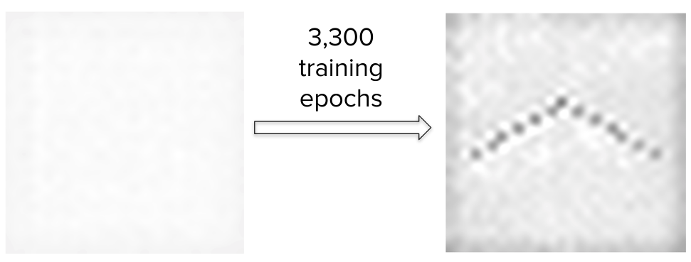
Figure 14: Sample image of propane generated by WGAN